Add stratigraphy from GeoTOP to CPT data

This example shows how stratigraphic layer boundaries from GeoTOP can easily be added to CPT data. This way, CPT parameters can easily be aggregated to get averages for geological units. For this example we are going to use a selection of CPTs in the area of the Utrecht Science Park (USP).

We will first import the relevant modules and plot the locations of the CPTs in the CptCollection.

import seaborn as sns
from matplotlib import pyplot as plt

import geost
from geost.bro import GeoTop
from geost.bro.bro_geotop import StratGeotop
from geost.analysis.combine import add_voxelmodel_variable


cpts = geost.data.cpts_usp()
cpts.header.gdf.explore(style_kwds=dict(color="red", weight=6))

Make this Notebook Trusted to load map: File -> Trust Notebook

Adding information from a voxelmodel

Any information from voxelmodels can be added. For this example we show how to add the stratigraphy from GeoTOP to the CPTs. First we read GeoTOP directly from the OpenDaP server for the USP area.

geotop = GeoTop.from_opendap(data_vars=['strat'], bbox=cpts.header.gdf.total_bounds)
print(geotop)

GeoTop
Data variables:
    strat    (y, x, z) float32 240kB ...
Dimensions: {'y': 12, 'x': 16, 'z': 313}
Resolution (y, x, z): (100.0, 100.0, 0.5)

As you can see, this prints a GeoTop instance along with the dimensions and resolution of GeoTOP. We can use this GeoTop instance to add the variable “strat” to the CPT data. This adds a column “strat” to the data object of the CptCollection. First, we must create a “depth” column in the CPT data because this is expected to be present in the data. We can use the column “penetration_length” for this. Below we add the variable and print the resulting column:

cpts.data["depth"] = cpts.data["depth"] 
cpts = add_voxelmodel_variable(cpts, geotop, "strat")
print(cpts.data['strat'])

0        1000.0
1        2010.0
2        3030.0
3        3100.0
4        5000.0
          ...  
73422    5000.0
73423    5060.0
73424    5070.0
73425    5120.0
73426       NaN
Name: strat, Length: 53994, dtype: float32

Note that some of the resulting values are “NaN” which occurs when a CPT falls outside of the 3D model extent. In this case, some CPTs are deeper than the maximum depth of GeoTOP. Now we could easily aggregate any CPT parameter according to the new “strat” variable. For example, make a boxplot of the average cone resistance (“qc”):

fig, ax = plt.subplots()
sns.boxplot(ax=ax, data=cpts.data.df, x="strat", y="cone_resistance", showfliers=False)
ax.tick_params(axis='x', rotation=45)

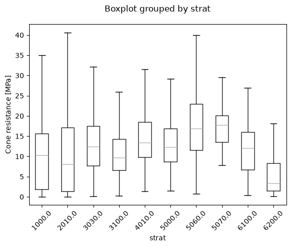
Each number on the x-axis represents a geological unit. However, these numbers are off course not really intuitive and knowing the corresponding geological unit is hard. GeoST provides the StratGeotop class which makes it easy to select desired stratigraphic units with or relabel the unit numbers in the plot above into more meaningfull names.

First, we select all the units that have been merged with the CPT data:

units = StratGeotop.select_values(cpts.data["strat"].unique())
units

[<HoloceneUnits.EC: 2010>,
 <ChannelBeltUnits.BEC: 6100>,
 <ChannelBeltUnits.CEC: 6200>,
 <OlderUnits.BXWISIKO: 3030>,
 <OlderUnits.BX: 3100>,
 <OlderUnits.KRBXDE: 4010>,
 <OlderUnits.DR: 5000>,
 <OlderUnits.UR: 5060>,
 <OlderUnits.ST: 5070>,
 <OlderUnits.PZWA: 5120>,
 <AntropogenicUnits.AAOP: 1000>]

This returns a list of enum types for each unit. An enum contains a “name” with corresponding “value”. Now, we can make a dictionary with both and replace the numbers with the names in the “strat” column. Let’s print the result and plot the figure again:

replace_dict = {unit.value: unit.name for unit in units}
cpts.data["strat"].replace(replace_dict, inplace=True)
print(cpts.data["strat"])

fig, ax = plt.subplots()
sns.boxplot(ax=ax, data=cpts.data.df, x="strat", y="cone_resistance", showfliers=False)
ax.tick_params(axis='x', rotation=45)

0            AAOP
1              EC
2        BXWISIKO
3              BX
4              DR
           ...   
73422          DR
73423          UR
73424          ST
73425        PZWA
73426         NaN
Name: strat, Length: 53994, dtype: object

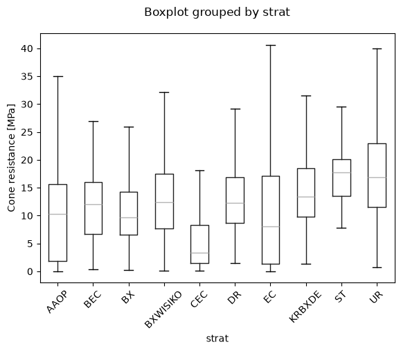
The x-axis in the plot now has some more meaningful abbreviations for geological units which can be found in the stratigraphic nomenclature. Most units belong to the “Boven-Noordzee Groep” (prefix “NU”). For example, the unit “EC” in the plot with the corresponding code can be found here.

The StratGeotop class can be used for all sorts of selections and groupings a user would like for further analyses.