Creating thickness maps from GeoTOP#

In this example we will retrieve GeoTOP from the OpenDAP server for an area around Delft and visualize the thickness of several geological layers and lithologies to gain a quick insight in how the subsurface in this area is built-up.

First, we import the GeoTop class from GeoST and retrieve GeoTOP data within the selected bounding box.

from geost.bro import GeoTop

# Load the GeoTOP model for the Delft area
geotop = GeoTop.from_opendap(bbox=(80000, 442000, 89000, 450000))

print(geotop)

GeoTop
Data variables:
    strat    (y, x, z) float32 9MB dask.array<chunksize=(82, 92, 76), meta=np.ndarray>
    lithok   (y, x, z) float32 9MB dask.array<chunksize=(82, 92, 76), meta=np.ndarray>
    kans_1   (y, x, z) float32 9MB dask.array<chunksize=(82, 92, 76), meta=np.ndarray>
    kans_2   (y, x, z) float32 9MB dask.array<chunksize=(82, 92, 76), meta=np.ndarray>
    kans_3   (y, x, z) float32 9MB dask.array<chunksize=(82, 92, 76), meta=np.ndarray>
    kans_4   (y, x, z) float32 9MB dask.array<chunksize=(82, 92, 76), meta=np.ndarray>
    kans_5   (y, x, z) float32 9MB dask.array<chunksize=(82, 92, 76), meta=np.ndarray>
    kans_6   (y, x, z) float32 9MB dask.array<chunksize=(82, 92, 76), meta=np.ndarray>
    kans_7   (y, x, z) float32 9MB dask.array<chunksize=(82, 92, 76), meta=np.ndarray>
    kans_8   (y, x, z) float32 9MB dask.array<chunksize=(82, 92, 76), meta=np.ndarray>
    kans_9   (y, x, z) float32 9MB dask.array<chunksize=(82, 92, 76), meta=np.ndarray>
    onz_lk   (y, x, z) float32 9MB dask.array<chunksize=(82, 92, 76), meta=np.ndarray>
    onz_ls   (y, x, z) float32 9MB dask.array<chunksize=(82, 92, 76), meta=np.ndarray>
Dimensions: {'y': 82, 'x': 92, 'z': 313}
Resolution (y, x, z): (100.0, 100.0, 0.5)

As you can see, geotop_delft is now an instance of GeoTop and provides a number of methods to make further selections and exports. We will make use of the GeoTop.get_thickness method.

We’d like to know the total thickness of clay layers in the area. Let’s first check the GeoTop lithology encoding, which can be accessed from the Lithology class or through downloading the reference list from the GeoTOP page on the BRO website. The code for ‘Clay’ in GeoTOP is 2, so we will use that in the get_thickness method as follows:

# Import the Lithology class to access GeoTOP lithological types
from geost.bro import Lithology

# Get the thickness of clay layers in the GeoTOP model and plot it
thickness_clay = geotop.get_thickness(geotop["lithok"] == Lithology.clay)
thickness_clay.plot.imshow(vmin=0, vmax=20)

<matplotlib.image.AxesImage at 0x7fbbe8242e40>

../_images/778429286db0b032c2a23a808b345c0eac88aba5fd1823f00c4d3e7aac11c455.png

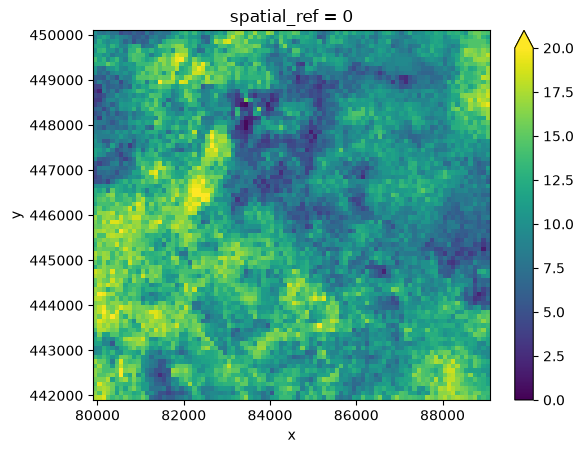
This shows the total thickness of all clay layers combined in the GeoTOP model. However, we are only interested in Holocene clay layers. The stratigraphic units defined in the StratGeotop class can be used to refine the selection. Alternatively, you can also reference the GeoTOP documentation and use the stratigraphic units numbering directly. We will use the StratGeotop class in this example:

# Import the StratGeotop class to access GeoTOP stratigraphic units
from geost.bro import StratGeotop

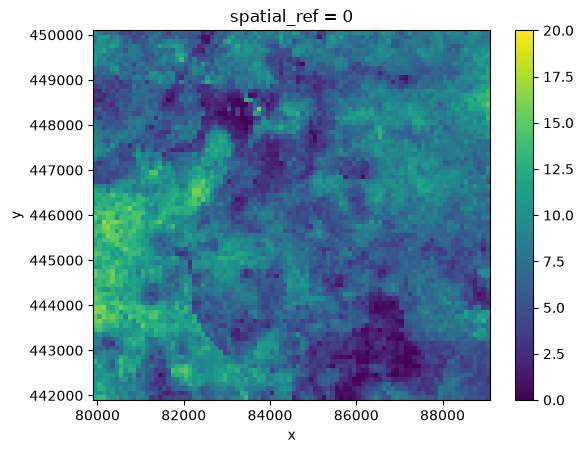
# Get the total thickness of clay in the Holocene stratigraphic units
thickness_clay_holocene = geotop.get_thickness(
    (geotop["lithok"] == Lithology.clay) & (geotop["strat"].isin(StratGeotop.holocene))
)
thickness_clay_holocene.plot.imshow(vmin=0, vmax=20)

<matplotlib.image.AxesImage at 0x7fbbd0f34e10>

../_images/a33339465826bb85baa9b22ac97c528c650cef241600a5402c76d6050eb0126f.png

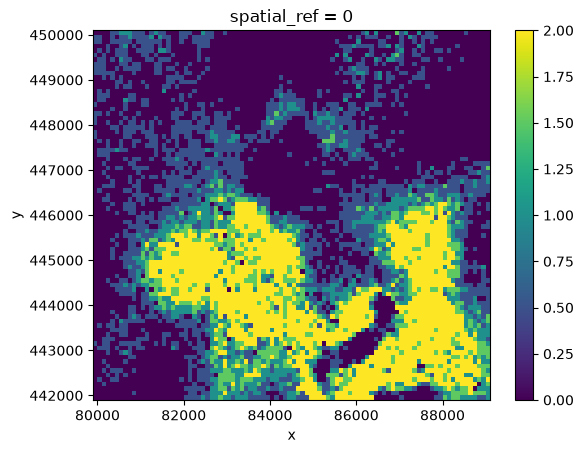
We can also get the thickness of, say, basal peat. The code for organic material is 1 and the stratigraphic unit we’re looking for is the Formatie van Nieuwkoop - Basisveen Laag, which is encoded as 1130.

# Get the thickness of basal peat
thickness_basal_peat = geotop.get_thickness(
    (geotop["lithok"] == Lithology.organic)
    & (geotop["strat"] == StratGeotop.select_units("NIBA"))
)
thickness_basal_peat.plot.imshow()

<matplotlib.image.AxesImage at 0x7fbbd0f77610>

../_images/b44aa2152680f3858ecfcc4203050be2b7b617ea08734d9a6013afba952312c9.png

Since the results are Xarray DataArrays, we can export them using rioxarray to geotiffs for sharing and viewing the results in GIS software for example.

# Export thickness_basal_peat to a GeoTIFF using rioxarray
thickness_basal_peat.rio.to_raster("thickness_basal_peat.tif")

Creating thickness maps from GeoTOP#

This Page