Data structures#

GeoST uses standardized internal data structures and data validation to ensure that the functionality that GeoST offers can always reliably be applied. This user guide section dives deeper into GeoST data structures.

Collection objects#

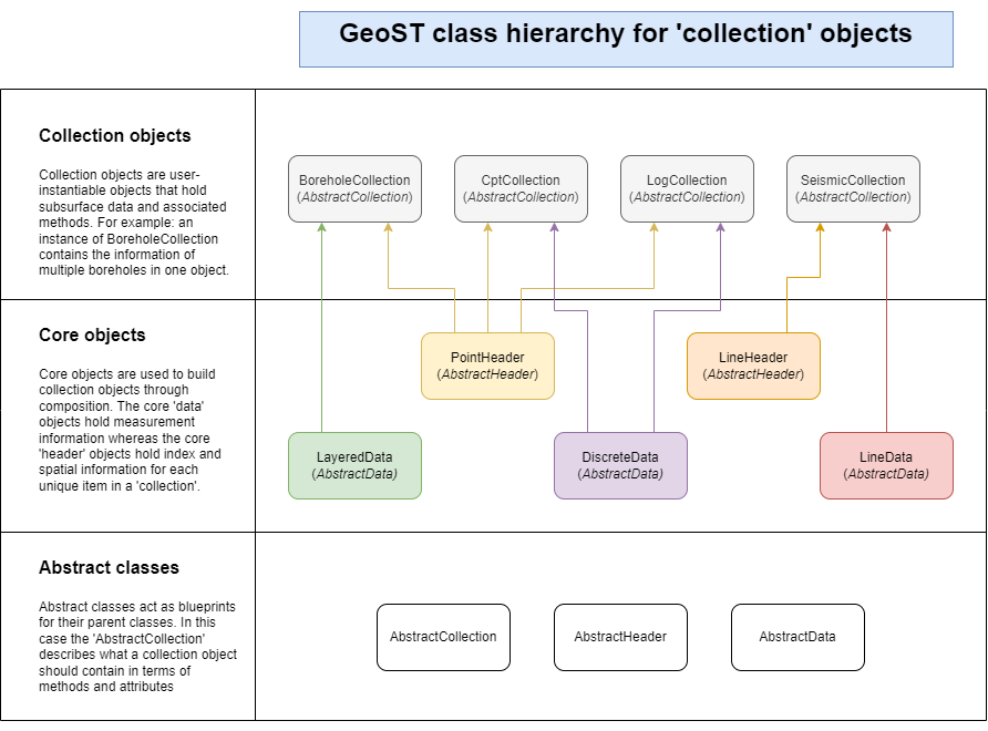
As shown in the first introduction to GeoST, data is held in so-called Collection objects, the core objects of GeoST, which contain header and data tables. Basically, the two can be described as:

the header table describes metadata and spatial information.
the data table contains the logged data.

The header and data tables have a one-to-many relationship: one survey (e.g. borehole) is one row in the header and multiple rows in the data.

Typically available types of subsurface data comprise point-like data such as boreholes, cpts, well logs and line-like data such as seismics, GPR, EM. Different data sources are related to specific Collection objects. For example, borehole data is held in a BoreholeCollection and CPT data in a CptCollection (see figure below).

GeoST object hierarchy

While working with a Collection, making selections may alter the header and data tables, Collections automatically maintain alignment between the two. Therefore, users can safely make selections and analyse the data while being sure of consistency. It is recommended to work with collections by default, unless you specifically only need to work with the header or data table. By default, read functions for different types of data return a collection (see: Reading data). So for example, reading sample data of boreholes available in GeoST shows that the resulting object is a BoreholeCollection. Additionally, we show that a Collection also contains horizontal and vertical spatial references.

import geost

# Load the Utrecht Science Park example borehole data
boreholes_collection = geost.data.boreholes_usp()

# boreholes_collection is an instance of BoreholeCollection and contains 67 boreholes
print(boreholes_collection)

# Print data types of header and data attributes
print(f"Data type header: {type(boreholes_collection.header)}")
print(f"Data type data: {type(boreholes_collection.data)}")

# Print the horizontal and vertical reference systems
print(boreholes_collection.horizontal_reference)
print(boreholes_collection.vertical_reference)

BoreholeCollection:
# header = 67
Data type header: <class 'geopandas.geodataframe.GeoDataFrame'>
Data type data: <class 'pandas.core.frame.DataFrame'>
EPSG:28992
EPSG:5709

Header table#

Header tables are a Geopandas GeoDataFrame instance and hold spatial information, in a “geometry” column, and metadata such as the surface level, end-depth and others. The geometry column of the header contains point geometries case of boreholes and CPTs and linestring geometries in for instance seismic data. Each entry (row in the Geodataframe) corresponds to one specific survey: e.g. one borehole or one seismic line.

A header table requires a bare minimum of data columns to be present to ensure that all built-in methods of a Collection can be used:

Column name	Validation criteria	Description
nr	Must be interpretable as string	Identification name/number/code of the point survey
x	Must be of numeric type (int or float)	X-coordinate
y	Must be of numeric type (int or float)	Y-coordinate
surface	Must be of numeric type (int or float) and higher than end depth	Surface elevation of the point survey in m +NAP
end	Must be of numeric type (int or float) and lower than surface elevation	End depth of the point survey in m +NAP
geometry	`shapely.geometry.Point` in case of point data	Geometry object of the survey location

The header is not limited to just these columns. Any number of columns can be added to give additional information on surveys. Some analysis methods may add information to the header. For instance, the method BoreholeCollection.get_area_labels has an argument include_in_header which, if set to true, adds a column with results to the header GeoDataFrame. Otherwise, it will return a separate DataFrame.

If you’re only interested in survey locations and/or metadata, it is adviced to directly work with the header object to avoid some additional overhead caused by a parent collection object (overhead is caused by checks of the header against data after every operation to ensure header/data alignment). Read functions for point and line data (see: Reading data) return a corresponding collection object by default, but you can assign only the header to a variable in order to continue with just the header data. See the example below.

# Load the Utrecht Science Park example borehole data and only assign the header data.
boreholes_header = geost.data.boreholes_usp().header

# Print the first rows of the header data.
boreholes_header.head()

	nr	x	y	surface	end	geometry
0	B31H0541	139585.0	456000.0	1.20	-9.90	POINT (139585 456000)
1	B31H0611	139600.0	455060.0	1.20	-23.00	POINT (139600 455060)
2	B31H0718	139950.0	455200.0	1.30	-271.20	POINT (139950 455200)
3	B31H0803	139675.0	455087.0	2.16	-4.84	POINT (139675 455087)
4	B31H0806	139684.0	455384.0	1.00	-49.50	POINT (139684 455384)

Data table#

Data tables are a Pandas DataFrame instance and hold all the logged data of any survey. In GeoST we mainly distinguish between “layered” and “discrete” data:

Layered data contains data that is logged in terms of layers (i.e. depth intervals over which properties are the same) with “top” and “bottom” information for each layer.
Discrete data contains data that is logged over discrete intervals (e.g. every 20 cm) with “depth” information for each measurement. One point or line survey (i.e. one row in the header) can be associated with multiple rows of data. E.g. a single borehole with 10 described layers is represented by one row in the header Geodataframe and ten rows in the data DataFrame.

Just like the header, a data table also requires a bare minimum of columns to be present to ensure that all built-in methods of a Collection can be applied. In case of “layered” data:

Column name	Validation criteria	Description
nr	Must be interpretable as string	Identification name/number/code of the point survey
x	Must be of numeric type (int or float)	X-coordinate
y	Must be of numeric type (int or float)	Y-coordinate
surface	Must be of numeric type (int or float) and higher than end depth	Surface elevation of the point survey in m
end	Must be of numeric type (int or float) and lower than surface elevation	End depth of the point survey in m
top	Must be of numeric type (int or float); starts at 0; is increasing	Elevation of layer top. The first layer always starts at 0 and increases downwards
bottom	Must be of numeric type (int or float); is larger than top; is increasing	Elevation of layer bottom

If the table contains inclined data, such as boreholes taken at a specific angle which means the x,y-coordinates of the top of a layer is not exactly at the same location as the bottom, the columns below must additionally be present:

Column name	Validation criteria	Description
x_bot	Must be of numeric type (int or float)	X-coordinate of layer bottom (only required if survey does not point straight down)
y_bot	Must be of numeric type (int or float)	X-coordinate of layer bottom (only required if survey does not point straight down)

In case the data table holds “discrete” data the columns below must be present to ensure that all built-in methods work. Note that the only difference is the “depth” column instead of the “top” and “bottom” columns.

Column name	Validation criteria	Description
nr	Must be interpretable as string	Identification name/number/code of the point survey
x	Must be of numeric type (int or float)	X-coordinate
y	Must be of numeric type (int or float)	Y-coordinate
surface	Must be of numeric type (int or float) and higher than end depth	Surface elevation of the point survey in m
end	Must be of numeric type (int or float) and lower than surface elevation	End depth of the point survey in m
depth	Must be of numeric type (int or float); is increasing	Depth where the measurement was taken

Also the data table is not limited to the columns above and all additional columns contain the actual data with measurements for each layer or at each depth.

If you’re only interested in the measurements and don’t need to work with geometries or any other additional header data, it is adviced to directly work with the data table to avoid some additional overhead caused by a Collection object (overhead is caused by checks of the header against data after every operation to ensure header/data alignment). The different read functions for data (see: Reading data) return a corresponding collection object by default, but you can assign only the Pandas DataFrame of the data table is returned to continue with just the data. See the example below. Some read functions, such as read_borehole_table provide the argument as_collection which defaults to True, but can be set to False to only return the data table in this example.

# Load the Utrecht Science Park example borehole data and only assign the data.
boreholes_data = geost.data.boreholes_usp().data

# Print the first few rows of boreholes data.
boreholes_data.head()

	nr	x	y	surface	end	top	bottom	lith	zm	zmk	...	cons	color	lutum_pct	strat_1975	strat_2003	strat_inter	desc
0	B31H0541	139585.0	456000.0	1.2	-9.9	0.00	0.20	K	NaN	None	...	None	ON	NaN	None	EC	NaN	[TEELAARDE#*#*#] ..........................
1	B31H0541	139585.0	456000.0	1.2	-9.9	0.20	0.60	K	NaN	None	...	None	BR	NaN	None	EC	NaN	[KLEI#*#*#] grysbruin.
2	B31H0541	139585.0	456000.0	1.2	-9.9	0.60	0.95	V	NaN	None	...	None	BR	NaN	None	NI	NaN	[VEEN#*#*#] donkerbruin.
3	B31H0541	139585.0	456000.0	1.2	-9.9	0.95	2.80	Z	NaN	ZMFO	...	None	GR	NaN	None	EC	NaN	[ZAND#*#*#] FYN TOT matig fyn# iets slib...
4	B31H0541	139585.0	456000.0	1.2	-9.9	2.80	4.20	Z	NaN	ZFC	...	None	BR	NaN	None	BXWI	NaN	[ZAND#*#*#] fyn# grysbruin.

5 rows × 32 columns

GeoST Accessors#

When you only need to work with one of the header or data tables, all the methods available in Collections are also available to the header GeoDataFrame and data DataFrame tables. This is achieved through so-called “accessors”. Under the hood, every Collection method also uses these accessors. Therefore, some methods specifically operate on the header table and others on the data table. The Collection then resolves the alignment between the two afterwards.

For the header table and associated header methods, the .gsthd accessor is available and for the data table, the .gstda accessor is available. Below we demonstrate shortly how these work by comparing the usage of Collection methods with those from the accessors.

# Create separate `collection`, `header` and `data` variables for the demonstration.
collection = geost.data.boreholes_usp()
header = collection.header
data = collection.data

Let’s first compare the usage of the select_within_bbox which is a method that operates on the header table. As the name suggests, this selects the surveys which are located within a specific bounding box extent. All we need to do to call this method on the “header” GeoDataFrame is using the .gsthd in between as shown below. After selecting from the header table, the .gsthd accessor remains available in the selection result for making further selections or chaining selections for example.

collection_select = collection.select_within_bbox(139_500, 455_000, 140_000, 455_500)
header_select = header.gsthd.select_within_bbox(139_500, 455_000, 140_000, 455_500)

print(collection_select)  # Selection result is a BoreholeCollection
print(type(header_select))  # Selection result is a GeoDataFrame

header_select.gsthd  # Selection result also has the gsthd accessor and methods available

BoreholeCollection:
# header = 14
<class 'geopandas.geodataframe.GeoDataFrame'>

<geost.accessors.accessor.Header at 0x7f7808d8c2d0>

For the data accessor, it works exactly the same way. We demonstrate this by comparing the slice_by_values method, which operates on the data table. Just like with the header, all we need to do to call this method on the “data” DataFrame is using the .gstda in between as shown below. After selecting from the data table, the .gstda accessor remains available for making further selections or chaining selections for example.

# Select boreholes which contain sand anywhere as the main lithology.
collection_select = collection.slice_by_values("lith", "Z")
data_select = data.gstda.slice_by_values("lith", "Z")

print(collection_select)  # Selection result is a BoreholeCollection
print(type(data_select))  # Selection result is a GeoDataFrame

data_select.gstda  # Selection result also has the gstda accessor and methods available

BoreholeCollection:
# header = 67
<class 'pandas.core.frame.DataFrame'>

<geost.accessors.accessor.Data at 0x7f77c829a8d0>

Every header and data method can be accessed through these accessors like it was shown in the examples above. Please see API Reference for the available methods through the .gsthd and through the .gstda accessors. For more detailed information on how the GeoST accessors work and the usage, please see the GeoST accessors page in this User guide.

Model data#

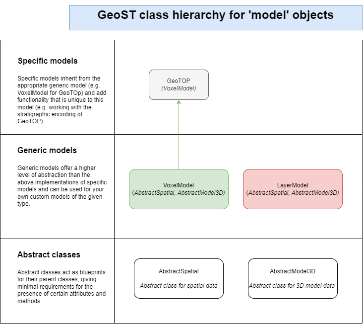
GeoST also supports working with model data and offers methods to combine these data with point and line data. Model data does not follow the same header/data approach as point and line data. Instead there are generic model classes, of which some have an implementation that adds specific functionality for that model. An example of this is the VoxelModel as a generic model class and GeoTOP being a specific implementation of a voxel model. GeoST currently supports the following generic models and implementations:

Generic models and implementations

VoxelModel: Class for voxel models, with data stored in the ds attribute, an Xarray.Dataset.
- Implementations: GeoTOP
LayerModel: Class for layer models, not yet implemented
- Implementations: None

GeoST vmodel object hierarchy

Voxel models#

The VoxelModel class stores data in the ds attribute, which is an Xarray.Dataset. A custom voxel model can be instantiated from a NetCDF file. For this, see the documentation of the VoxelModel.from_netcdf class constructor. An instance of VoxelModel offers basic methods for selecting, slicing and exporting models.

For more guidance on using a Voxel model within GeoST, see the BRO GeoTOP section in the user guide.