Event Set
This guidance provides support for preparing an event set to be used in FloodAdapt to calculate probabilistic flood maps, impacts, and risk. An event set consists of a set of events, defined by variables like surge, tide, and rainfall, and their occurrence frequencies. To see how FloodAdapt uses an event set to calculate risk, take a look at the FloodAdapt technical documentation on risk analysis, particularly the part about the probabilistic calculator.
The method described in this guidance is known as the Joint Probability Method (JPM). In the JPM, all types of hydro-meteorological events that may lead to flooding in an area of interest are identified. Subsequently, a representative set of (synthetic) events is selected, covering as much as possible the whole range of events that may contribute substantially to the overall flood risk. The likelihood of occurrence of each event is estimated from key statistics of the relevant flood drivers like rainfall, river discharge, and sea level.
Note that this guide focuses on non-hurricane events. For the derivation of a hurricane event set, which can be combined with a set of non-hurricane events, please see the comprehensive FEMA guide from 2023.
The joint probability method supports an event-based approach, like the one used in FloodAdapt. In this approach, synthetic events are generated and their occurrence frequencies are determined based on the joint probability of the variables defining the event (like surge and rainfall). Another approach is a time-series approach, where simulations are based on either a historical or synthetic time series of flood drivers. Probabilities do not need to be quantified in a time-series approach because correlations will be represented by the long time series. The time-series approach is easier to apply and easier to standardize, but requires long good-quality records of all relevant flood drivers, which are usually not available.
Steps to prepare an event set
This guide is organized around key steps in preparing an event set.
Identify flood drivers and define variables
Determine the flood drivers that have a significant impact on the flood risk in the area (e.g. rainfall, river discharge, sea levels), and select appropriate variables that best represent the characteristics of the identified flood drivers.
Calculate probabilities of variables
Calculate the probability distribution of the flood driver variables.
-
Calculate correlation between variables and the joint probability of occurrence of the flood driver variables.
Select events and calculate their frequencies
Select a set of events (defined as a combination of flood driver variables) and quantify their occurrence frequencies.
Format the events for FloodAdapt
Prepare the set of events (event specs and frequencies) in the format required for FloodAdapt.
Step 1 - Identify flood drivers and define variables
The initial step in setting up a probabilistic flood risk assessment involves identifying the most relevant flood drivers in the project area. In coastal zones, floods may be caused by (combinations of) intense rainfall (pluvial flooding), high river discharges (fluvial flooding), groundwater tables rising above the ground surface (groundwater flooding), and high tides, storm surges, and waves (coastal flooding). In a probabilistic analysis, these flood drivers are represented by variables that quantify a specific characteristic of the flood driver, such as daily rainfall or peak storm surge. These variables are sometimes referred to as “stochastic variables” or “random variables,” acknowledging the fact that they can take on a range of values that have probabilities of occurrence/exceedance associated with them.
The choice of the most suitable variable to represent a flood driver depends on the system under consideration. For example, for an assessment of a storm sewage system, a suitable variable may be the 15-minute or 1-hour rainfall, whereas for larger catchments the daily rainfall or multi-day rainfall is more relevant. For the design of river embankments, the peak discharge is a suitable choice, whereas for the design of a reservoir the total volume of flow during the entire flood event is also relevant. In some cases, it may be worth considering representing a flood driver with multiple variables. For example, river discharge can be represented by a combination of peak flow and flow volume.
Limiting the number of variables in a probabilistic flood risk assessment is crucial due to the exponential increase in the required model simulations, which can impact practical feasibility and computational resources. Consider a scenario where only two variables—rainfall and storm surge—are selected, each with five possible realizations. This setup yields 25 possible combinations (5×5), necessitating 25 model runs to assess flood conditions and impacts. This number of simulations is generally manageable. However, increasing the variables to four, each with five realizations, results in 625 possible combinations (5×5×5×5), significantly increasing the simulation time. If the number of variables increases to six, this leads to a staggering 15,625 combinations (5^6), which may not all need simulation but illustrate the potential scale of the assessment.
While a comprehensive analysis ideally covers all relevant flood events, practical constraints often necessitate a balance. The choice of the number of model simulations is a trade-off between accuracy and simulation time. It is important to understand the relationship between the flood drivers and flood response, which may come from existing knowledge of the area or from exploratory simulations with a Hydrologic/Hydraulic (H&H) model. Conducting a sensitivity analysis with the H&H model for each candidate variable allows quantification of the sensitivity of the flood hazard and impact. Variables for which this sensitivity is relatively small can be replaced by a constant value, reducing the complexity of the analysis and computation times. For example, while the peak river discharge is a critical variable if a project area is along a river, in coastal areas where water levels are dominated by the sea, a constant river discharge might suffice, verified through sensitivity analysis to assess its impact. This demonstrates the essential balance between accuracy and practicality in setting up probabilistic flood risk assessments, aiming to include as many variables as necessary but as few as possible to maintain manageability and effectiveness, particularly if scenarios need to be re-evaluated frequently due to changing climate conditions or socio-economic factors.
Step 2 - Calculate probabilities of variables
Flood events are described as a combination of realizations of the selected flood driver variables. For each event considered in the probabilistic analysis, the probability of occurrence is needed to be able to quantify the contribution of such an event to the overall risk. The event probabilities are derived from probabilities of the flood event variables. In some cases, probability distributions of variables are readily available. NOAA, for example, offers nation-wide statistics on rainfall (NOAA rainfall). In other instances, probabilities need to be derived either from gauge records or from expert judgement.This section focuses on deriving probabilities/statistics from gauge data.
The main steps in deriving (joint) probabilities of the flood variables are:
Data gathering and validation - this step involves collecting and ensuring the quality of time series of the variables for which we want to derive probability distributions
Correcting for non-stationarity - this step involves correcting for changes in the system or trends which would make distribution fitting techniques invalid
Extreme value analysis- this step fits distributions to the extreme tails of the flood variable distributions
Combining statistics of extreme events and average conditions - this step creates a distribution that is correct for both average values of the variables and extreme values
Data Gathering and Validation
Data gathering is a critical step in flood risk assessment. Important considerations include the record length, temporal resolution, number of stations, and data validation processes. Long records are preferable as they provide more comprehensive information on “extremes,” which are crucial for analyzing flood risks.
Record Length: Longer records are more valuable because they include more rare events, which are important for understanding the full range of possible scenarios. They also allow for more robust statistical analyses.
Temporal Resolution: The temporal resolution of the data should align with the scale of the hydrological processes being modeled. For urban drainage studies, minute-by-minute data may be necessary, whereas for river basin studies, daily values may suffice.
Number of Stations: Gathering data from multiple stations is generally preferred over using data from only one station. This provides valuable information on spatial variability. Furthermore, comparing data between nearby stations is an excellent way to validate data.
Data Validation: It is critical to validate the data to ensure its accuracy and reliability. This involves checking for anomalies or errors, such as outliers that might indicate data recording errors, especially for extreme values.
Dealing with Non-Stationarities
Sometimes, data is collected from a period when the system under consideration was significantly different from the current situation. As a result, the recorded time series may be non-stationary, meaning that probabilities of occurrence/exceedance can change over time. Various factors could cause changes in the system over the years, including climate change, sea level rise, urbanization, morphological changes, and human interventions like reservoirs. In such cases, caution is needed when using this data, as it could lead to over- or underestimation of current flood risk. One option is to discard earlier data, but this removes potentially useful information and may leave too little data to derive reliable statistics. Alternatively, ‘corrections’ can be applied to make the data set (approximately) stationary again. The aim of these corrections is to estimate what the observed time series would have looked like if the system conditions had been the same as they are today.
For coastal systems, corrections for sea level rise are almost always necessary. Due to sea level rise, the exceedance probabilities of sea water levels increase over time, making early observations non-representative of current conditions. A simple correction is to add the amount of observed sea level rise since year Y to all observations from that year. For instance, if sea levels have risen by 0.5 ft since 1990, all water levels observed in 1990 should be increased by 0.5 ft to reflect current conditions. This adjustment requires an understanding of the extent of sea level rise, which is complicated by year-to-year fluctuations that can obscure the long-term trend. To address this, a trend line might be fitted through the data, although this process can be somewhat subjective.
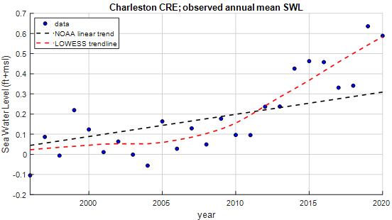
Figure 1 illustrates annual average observed sea water levels from 1996-2020 in Charleston, SC (blue dots), with the black line representing a linear trend line as derived by NOAA (NOAA SWL trend), and the red line showing a non-linear trend line using the LOWESS method (Cleveland, 1979). The estimated average sea level in 2020 differs by approximately 0.3 feet between the two methods, indicating that the choice of method can significantly influence the estimated flood risk. The linear fit does not account for the notable increase in sea water levels observed since 2014, suggesting the LOWESS fit might be more appropriate. However, this increase could be an anomaly; a similar sharp rise occurred in the 1940s, but by the late 1950s, the data returned to align with the linear trend. This variability demonstrates that past sea level rise is uncertain, and it may be prudent to consider both trend lines when assessing potential impacts on flood risk.
In cases like these (sea level rise, implementation of a reservoir) the recorded time series are clearly non-stationary and the cause of the non-stationarity is known. In other situations, there may be an observed trend for which it is unclear if this is due to a change in the system or if it is merely a coincidence. In that case, statistical tests can be applied to assess the likelihood of the trend being just a coincidence. IExamples of such tests are the Mann-Kendall test (Mann, 1945; Kendall, 1975) and the Wilcoxon-Mann-Whitney test (Wilcoxon, 1945; Mann and Whitney, 1947).
Extreme Value Analysis
Extreme value analysis is used to derive statistics of the “extremes” in a record, based on limited information. For floods, this is important because often it is the extreme values of the flood variables that lead to a flood event, but these occur infrequently. Extreme value analysis involves selecting peaks (either annual maxima or peaks over threshold) and fitting them to appropriate probability distribution functions.
Selection of peaks
The first step in the process is to select a subset of the record that contains the extreme variable values. This is generally either the set of highest recordings in each year, known as annual maxima (AM) or the set of recordings that exceed a user defined threshold, known as peaks over threshold (POT).
For annual maxima the selection can be done for each calendar year, but it can also be done for a “water year” which may have a different start date than January 1st. The start of the water year should preferably be chosen in a season where little or no extremes are expected. This way, the chance is small an extreme event occurs right around the start of the year and is selected as the annual maximum for two consecutive years (for example, if high peaks occur on December 31st and January 1st that are caused by the same meteorological event).
For peaks over threshold, only a single value per event should be selected. So, for example, if a river discharge exceeds the threshold for five consecutive days, these can all be considered part of the same event and only the highest observed discharge during these five days should be selected as the peak discharge. It is recommended to define a time window during which only one peak can be selected to assure the selected peaks all represent independent events. The size of the window depends on the system/process under consideration. For a small mountain stream, a window of one or two days may suffice, whereas for a large river basin (> 25,000 square miles) the window should be at least 10 days. A suitable choice of the threshold in a POT analysis also depends on the system under consideration. A lower threshold has the advantage that a larger number of peaks is selected which decreases the uncertainty in the probability distribution function that is subsequently derived from the selected peaks. On the other hand, it also results in lower peaks to be selected, which may be less representative of the extremes for which probabilities need to be derived, which may not be representative for the extremes for which statistics are derived. A pragmatic strategy is to choose the threshold in such a way that the number of selected peaks is equal to the number of years. This strategy is sometimes referred to as “Annual Exceedance” (AE). Note that this series is not the same as AM, even though they both have the same number of peaks.
Selection of a probability distribution function
The next step is to select a probability distribution function that will be fitted to the selected set of peaks. According to the extreme value theorem, the set of maxima of intervals of a fixed length (such as a year) has a Generalized Extreme Value (GEV) distribution. POT data follows a Generalized Pareto Distribution (GPD). Both GEV and GPD are three-parameter distribution functions with a location-, scale- and shape-parameter.
The GEV and GPD are generalized distributions of which other probability distributions are special cases: Gumbel, Fréchet and Weibull (GEV) and exponential and Pareto (GPD). The value of the shape parameter determines which of the underlying distributions is applicable for the data. If the shape parameter is approximately equal to zero, the Gumbel (GEV) and exponential (GPD) distribution functions should be used. If the shape parameter differs from zero, the Fréchet and Weibull (GEV) and Pareto (GPD) should be used. The value of the shape parameters can be derived from the selected set of peaks (see later this section on fitting distribution functions).
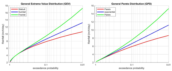
Figure 2 shows examples of these distribution functions for daily rainfall. The rainfall is plotted against the corresponding exceedance probability on a semi-logarithmic scale. It shows that the two distribution functions for which the scale parameter is equal to 0 (Gumbel and exponential) are straight lines on this scale. The Weibull distribution is curved “downward”, while the Fréchet distribution is curved “upward”. Similar upward and downward curves can be seen for the GPD (right plot); in both cases the distribution function is called the Pareto distribution. According to the theory, only the GEV and GPD or one of the underlying probability distribution functions (Gumbel, Fréchet, Weibull, exponential and Pareto) should be used to fit the set of selected extremes. In practice, however, other probability distribution functions are used as well. For example, the Log-Pearson Type 3 was adopted by US federal agencies for applications in flood frequency analysis.
The graphs in Figure 2 show the probability of exceedance of annual maxima (left) and peaks over threshold (right) data. The exceedance probability of AM also represents the annual exceedance probability of the variable for which the distribution function was derived. For POT data, this is not the case because the number of peaks in a POT data set can be larger or smaller than the number of years. To convert to an annual exceedance probability, the derived exceedance probabilities of POT data must be multiplied by the average number of exceedances of the selected threshold in a year (denoted \(\lambda\)). Parameter \(\lambda\) can be estimated by dividing the number of selected peaks by the number of years in the record. Note that \(\lambda\) is a frequency of occurrence (per year). Multiplication of this frequency with a probability of exceedance from the POT data results in a frequency of exceedance.
The terms “probability” and “frequency” are often used interchangeably to quantify the likelihood of a specific event occurring within a defined period. These two terms are similar, but not the same. Probability refers to the chance that an event will occur in a fixed period, typically a year. Frequency refers to how often such an event will occur on average during a fixed period. For example, at some location the probability of more than 5 inches of rainfall in a day may be estimated at 1/20 per year. That means each year there is a probability of 1 in 20 that more than 5 inches of rainfall is recorded in a day. In this case, the frequency is also equal to 1/20 per year, indicating such an event will occur on average once every 20 years. However, for events that occur more often, probability and frequency differ. For example, an event with more than 2 inches of rainfall in a day may occur on average twice per year. That means such an event has a frequency of 2 (per year). The probability of such an event happening in a year will be less than 1 since probabilities are, by definition, between 0 and 1. Probability is a quantification of the chance of such an event occurring at least once in a year, whereas frequency is a quantification of the number of times such an event occurs on average in a year. For very rare events, probability and frequency are (approximately) equal, because such events are not expected to occur more than once per year.
Fitting probability distributions
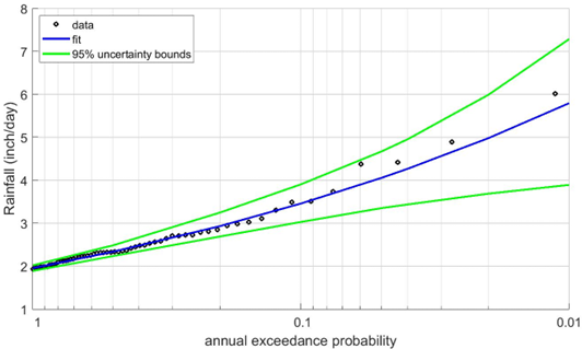
The next step is to fit the selected distribution function to the set of extremes (AM or POT). This means the parameter values of the distribution function are chosen such that key statistical characteristics of the distribution function correspond as much as possible with those of the set of extremes. There are several methods for deriving the parameter values, such as the maximum likelihood method, the method of moments, probability weighted moments and L-moments. Such methods are available in computational programming languages like Matlab, Python and R. Alternatively, dedicated software for flood frequency analysis can be used such as PeakFQ. In principle, any of these methods will do, but it is worth considering applying several methods to verify which one provides the best fit. There are statistical methods to quantify the goodness-of-fit like the Kolmogorov-Smirnov test, the Chi Square test or Anderson-Darling test. Each of these tests compares key characteristics of the data set with the fitted distribution function; smaller differences imply a better fit. The outcome of such a test could be that a fit is “rejected”. In that case an alternative distribution function and/or fit method should be considered. The fact that there are different tests to choose from indicates there is some subjectivity involved in determining the “best” fit. It is recommended to also visually compare the fitted distribution function with the data, similar to the example of Figure 3. If the visual fit is not to satisfaction, a different distribution function and/or different fit methods should be considered.
Combining statistics of extreme events and average conditions
In flood risk analysis, the extremes as described in the previous section are the most relevant subset of the data. However, in areas with compound flooding, extremes of flood drivers do not necessarily coincide in time. For example, high intensity rainfall may occur during a period with negligible, low or moderate storm surge, and vice versa. This may result in a (substantially) different flood hazard compared to when both flood drivers are high/extreme. For a flood risk analysis with multiple flood drivers it is therefore necessary to also consider events where only a subset of the flood drivers is extreme. This means it is required to also derive probabilities of moderate/average conditions of flood drivers.
Similar to the extreme value analysis of the previous section, probability distribution functions can be selected and fitted to the available data set. The main difference is that in this case the entire data record is used instead of a small selection. With this larger data set, the use of an empirical distribution may be more practical than fitting a parametric probability distribution function. The advantage of using an empirical distribution functions is that it is relatively straightforward to derive and does not involve subjective choices of a distribution function and fit method. The empirical distribution is a direct reflection of the data set. For example, if a daily rainfall depth of 0.1 inch is exceeded in 12% of all days in the record, this means the exceedance probability of 0.1 inch/day in the empirical distribution function is estimated to be 0.12. So, by simply counting the number of exceedances of each threshold of interest and dividing by the total number of recordings, the empirical probability is obtained.
To derive the empirical probability distribution, sort the data in descending order. The largest value has an empirical probability of exceedance of 1/(n+1), where n is the total number of recordings. The second largest value has an empirical probability of exceedance of 2/(n+1), the third largest has an empirical probability of exceedance of 3/(n+1), and this continues all the way down to the smallest value with an empirical probability of exceedance of n/(n+1). Note that these are probabilities per time step of the time series. So, in case of a daily rainfall time series, these are exceedance probabilities per day. These can be translated to exceedance frequencies per year by multiplication with 365 (i.e. the number of days per year). Similarly, derived empirical probabilities of tidal peaks should be multiplied with 705 (i.e., the number of tidal periods in a year) to derive exceedance frequencies per year.
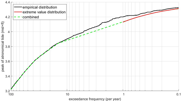
The variable of interest now has an empirical distribution function, quantifying probabilities of all observed values, and an extreme value distribution function, quantifying exceedance probabilities of extremes. So, for the highest observed values in the record there are two probability estimates available. Ideally, these two probability estimates are the same, but this is often not the case. Especially for variables for which high peaks typically occur in clusters, there will most likely be a substantial difference in the two probability estimates due to the differences in the way these two probabilities were derived. Figure 4 shows the empirical probability distribution (black line) and fitted extreme value distribution (red line) of the tidal peaks at an example location. It shows the exceedance frequencies according to the empirical distribution are higher than those according to the extreme value distribution function. The green dashed line shows a pragmatic way to connect the two distributions and combine them into a single probability distribution function. An alternative approach could be to “lift” the extreme value distribution such that is better connects with the empirical distribution. Such methods may seem like they are corrupting the results, but it is a necessary work-around to combine two distributions that are based on different approaches. The first approach (“each tidal peak should be included”) is valid for average/moderate conditions, whereas the second (“only the highest peak of each event is included”) is valid for extreme events.
Step 3 - Calculate joint probabilities
Event probabilities are the joint probabilities of the variables that define the event. If the variables are mutually independent, the joint probability can be calculated as the product of the the probabilities of the individual variables. However, some variables may be impacted by the same hydro-meteorological processes, which means they are not independent. For example, a storm event may cause both high storm surges and high rainfall intensities. In that case, high values of rainfall and storm surge are more likely to coincide, which means rainfall and storm surge are not independent. This needs to be accounted for when estimating event probabilities.
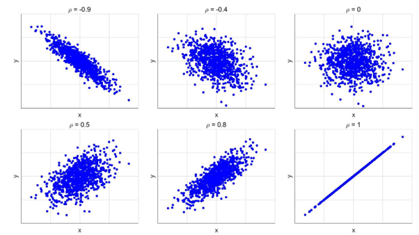
Statistical dependence between two or more variables can be quantified with Pearson’s correlation coefficient, \(\rho\), which can take any value in the range from -1 to 1. A value of 0 indicates two variables are independent, which means the value of one variable provides no information on the likelihood of the value of the other variable. If \(\rho\) deviates substantially from 0, the variables are dependent. Positive values of \(\rho\) imply that high values of one variable usually coincide with high values of the other variable, and similarly that low values generally coincide as well. Negative values of \(\rho\) imply that high values of one variable usually coincide with low values of the other variable and vice versa. Figure 5 shows samples of hypothetical variables x and y for six different values of Pearson’s correlation coefficient.
Pearson’s correlation coefficient assumes a linear relation between the correlated variables, which is not always the case. If two variables are perfectly correlated, but their relation is non-linear, the value of \(\rho\) will be less than 1, indicating non-perfect correlation. This is one of the reasons why a rank correlation may be preferred over Pearson’s correlation coefficient. The two most well-known options are Spearman’s and Kendall’s rank correlation coefficients. Similar to Pearson’s correlation coefficient, these two rank correlation coefficients take on values between -1 and 1.
Even though the correlation coefficient generally is an informative measure of statistical dependence, it does not provide the complete picture on dependency structures. In some cases, for instance, the dependence between variables is higher for extremes than for moderate events due to a common cause that is especially profound during extreme events. This phenomenon is sometimes observed in discharge records of two neighboring rivers. If one river experiences extremely high discharges, this is likely to be the result of an exceptional rainfall event that may also cause high discharges in the other river.
An effective approach to incorporate these types of correlation structures is the use of “copula functions” or “copulas”, which model the dependence structure of two or more random variables. A multivariate distribution function is then constructed using the individual probability distribution functions of the variables in combination with the copula. One of the key advantages of this method is that the derived individual probability distributions are preserved, which is not necessarily the case with alternative methods for deriving multivariate statistics.
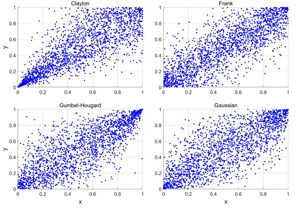
Figure 6 shows example realizations of copula variables x and y for four different copulas: the Gumbel-Hougard, Frank, Clayton and Gaussian copula. In each case, the correlation coefficient is equal to 0.8, but there are differences in the overall dependence structure. Application of the Gumbel-Hougard copula results in strong dependence for values of x and y close to 1. In other words, if a sample of the first random variable (x) is relatively large, the accompanying sample of the second variable most likely is relatively large as well. The Clayton copula, on the other hand, generates a stronger dependence structure for low values of x and y. In that respect the Frank copula and the Gaussian copula are more symmetrical, where the latter shows stronger correlation in the extremes (both left and right).
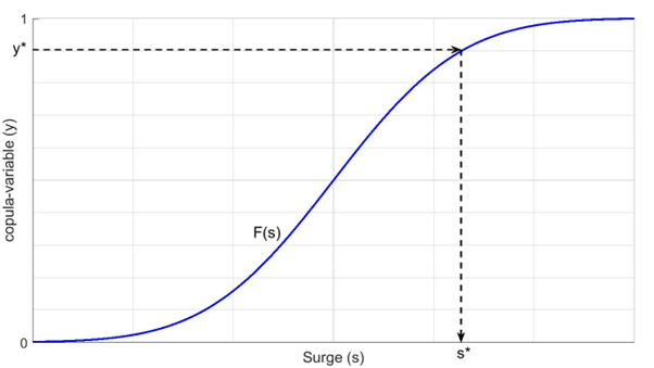
Copula variables are uniformly distributed over the interval between 0 and 1. Hydro-meteorological variables like rainfall, river discharge or water level are typically not uniformly distributed and can take on values outside the interval between 0 and 1. Therefore, in order to use the copula to model dependency between hydro-meteorological variables, a statistical transformation is applied. This transformation is done based on “equal probability of exceedance”. The transformation process is illustrated in Figure 7.
Since copula-variables x and y are correlated, the corresponding real-world variables (e.g. rainfall, surge) will be correlated as well. This way, a set of correlated samples of storm surge and rainfall can be generated. Conversely, the copula function and transformations can also be used to compute the probability of an event of, for example, a river discharge of more than 5,000 cfs in combination with a storm surge of more than 2 feet. To do this, these thresholds of discharge (5,000 cfs) and storm surge (2 feet) need to be translated to their corresponding copula-parameters x and y, using their respective probability distributions.
Figure 6 showed patterns of four copulas, but there are many other copulas available, covering essentially any correlation pattern imaginable. A copula needs to be selected that best matches the observed data. Plotting of observed joint occurrences of correlated variables may reveal which copula(s) best describe the correlation between the variables involved. For example, if the data indicate the dependency increases for large values, the Gumbel-Hougard copula is a possible candidate, whereas if the dependency increases for low values, the Clayton copula is a possible candidate. Another strategy is to try out a large set of copulas and verify which one provides the best fit of the data. There are several statistical tests available that quantify the goodness-of-fit of the copula to the data, similar to the goodness-of-fit tests for extreme value distribution functions. Such methods are available in computational software packages like Python and R.
Step 4 - Select events and calculate their frequencies
When considering the selection of events, it is important to remember its purpose: the set of events will be used to calculate return period flooding and expected annual damages. The key to event selection is to ensure that the set of events is sufficient to reliably (consistently) estimate these important variables. There are two primary ways to select events and estimate their occurrence frequencies. One is to use a Monte Carlo approach, which is most recommended when there are a lot of variables that influence the flooding. The second is numerical integration, which is is more straight-forward and advantageous (in terms of required number of events) when the number of variables is limited to two - which may be the case for many areas.
With Monte Carlo sampling, a set of synthetic events is generated from the joint probability distribution of the event variables. This can be considered a representative set of possible events that may occur. For example, if an event with a joint occurrence of a peak river discharge between Q1 and Q2 and a peak sea water level between H1 and H2 has a probability of 0.05 per year according to the joint distribution, the sampling will lead to 5% of the simulated years containing an event in this range. However, since the sampling process is random by nature, the resulting percentage can also be lower or higher.
In a Monte Carlo Simulation, events are sampled directly from the multivariate probability distribution function of the flood drivers. The event set for FloodAdapt would consist of this set sampled events. The associated probability for each event is set equal to \(1/n\), where \(n\) is the total number of sampled events. Note that this is not the actual probability of each event. However, by applying this probability as input in FloodAdapt, the computation of flood probabilities will be according to the Monte Carlo Simulation method. In other words, the computed probability of flooding will be equal to the number of sampled events leading to flooding, divided by the total number of simulated events.
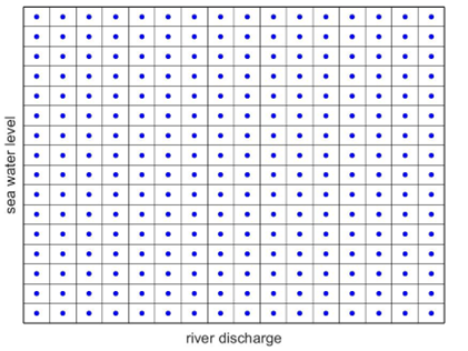
With numerical integration, the range of potential combinations of flood drivers is discretized in an n-dimensional computational grid (n being the number of flood drivers), so that all combinations are considered. Figure 8 shows an example for two flood drivers: river discharge and sea water level. In Figure 8, each rectangular grid cell has a center point, representing a single event with that combination of sea water level and river discharge. The event occurrence frequency is then taken as equal to the joint occurrence frequency of the variables. The range of variables that should be included, and the spacing of the computational grid, depend on when the values of interest (flooding probabilities and risk) stabilize. Extreme combinations of variables that have a very low occurrence frequency may not contribute a noticeable amount to flood probabilities or risk. Similarly, high-frequency low values of the variables that do not lead to flooding may also be negligible. For the latter, it is important to consider if they will still be negligible under future conditions before omitting them from the event set.
Both for Monte Carlo and for numerical integration, more events means better accuracy, but comes at a computational cost. For the Monte Carlo approach, a higher number of samples leads to better accuracy. For the Numerical Integration approach, a finer discretization of the variables leads to better accuracy. In each case, simulations with FloodAdapt can be done to assess the trade-off between number of events and accuracy of the risk and flood probability metrics.
Step 5 - Format the events for FloodAdapt
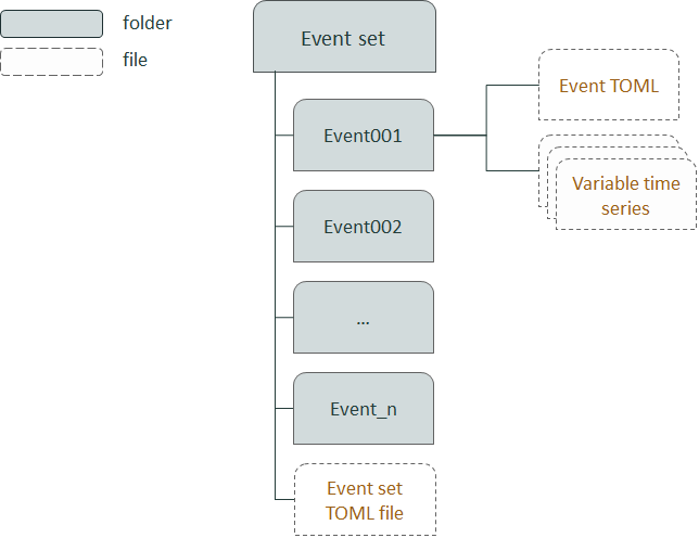
Once you have selected events and calculated their occurrence frquencies, they must be put in the correct format for FloodAdapt. Figure 9 shows the overall structure of the event set folder. The folder contains a sub-folder for each event in the event set and an event-set TOML file that gives the event names (which should align with the folder names) and the occurrence frequencies of the events. Each event folder should contain an event TOML file defining the event, and the time series (for the event duration) of the flood variables. More details about the event folder contents and the event set TOML file are given below.
Event folder contents
Each event folder must contain a TOML file, with the name [EVENT_NAME].TOML, where [EVENT_NAME] should be replaced with the name of your event (which is also the name of the event folder). For example, if your event is called myEvent001, then the event folder should be called myEvent100, and the TOML file should be called myEvent001.TOML. In addition, the event folder must contain a time series file (CSV format) for each of the event variables that are varying over the duration of the event. Figure 10 shows the contents for an event named event_001.
The time series CSV files are two-column files that contain a datetime in the first column and the variable value in the second column. The units of the variable will depend if you are working with imperial or metric units:
- Rainfall - inches/hour (imperial) or mm/hour (metric)
- Tide - feet+MSL (imperial) or meters+MSL (metric)
- Surge - feet (imperial) or meters (metric)
- River discharge - cubic feet per section (imperial) or cubic meters per second (metric)
- Wind - knots (imperial) or m^3/s (metric)
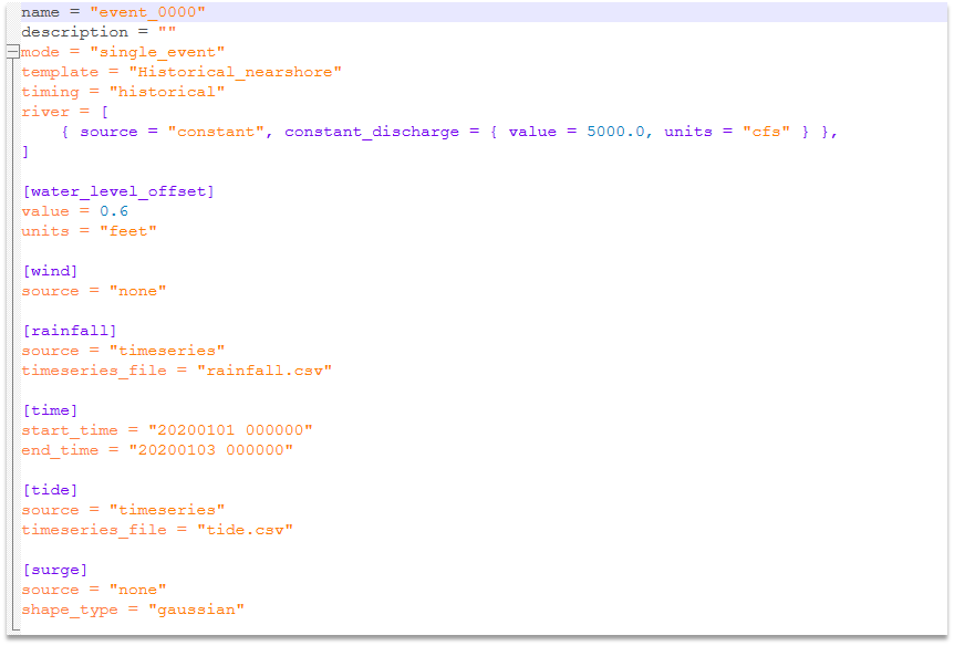
The TOML file specifies the event. Figure 11 shows the template for an event TOML file, which includes forcing fields for river discharge, wind, rainfall, tide, and surge. In this example, there are two probabilistic event variables: rainfall and total sea water level (which includes both tide and surge). The river discharge is treated as a constant and wind is omitted because its effects are already accounted for in the total water level (which includes surge). Because the total water level variable includes both tide and surge, the surge variable is omitted (set to “none”) and the total water level time series is used for the “tide” field. A couple of notes about the event specifications:
- All potential flood drivers must be defined, even if they are set to zero or none. For example, in Figure 11, the wind is set to “none”. Similarly, the discharge is set to “constant” because it is not treated probabilistically in this event set.
- Although the events are synthetic they use the “Historical_nearshore” template because the event variables are being represented by time series like a historical event. This means that a start time and end time must be given. These can be anything in the past, as long as the duration matches the duration in the variable time series files.
Event set TOML file
The event set folder must contain an event set TOML file. This file will specify the names and occurrence frequencies of all of the events in the set. Every event specified in this TOML file must also have an associated event folder. Figure 12 shows an example of a TOML file for a set named “probabilistic_set”.
The required fields are:
- name - this should also be the name of the event-set folder
- description - this can be anything
- mode - this should be set to “risk”
- subevent_name - this is a list of the events for which event folders have been created
- frequency - this is a list of occurrence frequencies for the events in the subevent_name list
Once the event set folder is created, you can reference it in the database builder configuration file and it will be included in the FloodAdapt database so users can calculate risk and risk-reduction benefits of adaptation options.
