Synthetic events
When the user selects the “Synthetic” option from the Events tab, they will see the event template window shown in Figure 1. This window allows the user to input synthetic time series for:
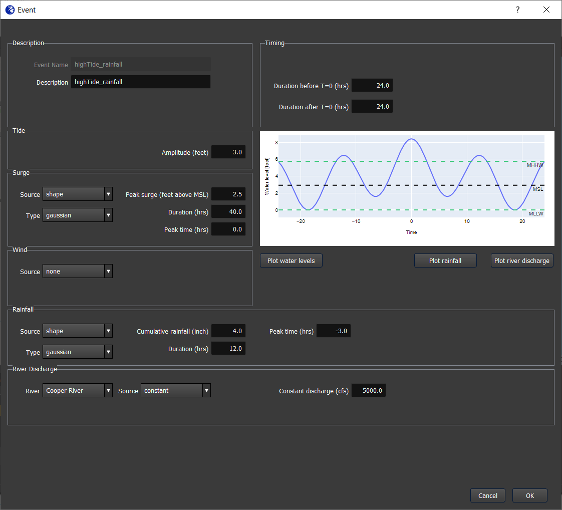
Duration of the synthetic event
The duration is specified by the user in the “Timing” block. The start time is given as a duration before T=0 (in hours), and the end time as a duration after T=0 (hours).
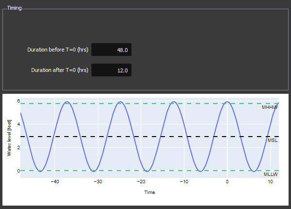
The time T = 0 is an arbitrary moment when the tide is at its crest. It is essentially a ‘reference time’ to define the duration of an event, and to specify other forcing variables in relation to. Figure 2 shows an event with a duration 48 hours before and 12 hours after T=0. You can see the crest of the tide occurs at T=0, and the event runs from 48 hours before until 12 hours after this moment.
Water levels - Tide + Surge
For a synthetic event, the water level is treated as a sum of the tidal and surge components, which are specified separately.
The tide is entered as an amplitude above or below mean sea level. The window will open with a default value that was configured when the FloodAdapt system was set up.
The surge timeseries is specified as a Gaussian curve. The user specifies the peak surge, the duration of the surge, and the timing of the peak relative to T=0. Figure 3 shows an example how a user can adjust the surge timing. The figure shows three panels. The top panel has the tide set to zero, so the timeseries of the surge alone can be viewed. The surge is set as a Gaussian curve with a peak value of 6 ft, and a duration of 12 hours. The second panel shows the timing of the peak surge at -5 hours, with the tide set back to its default value of 3 ft. This is 5 hours before T=0, when the tide was not at its crest. The third panel shows the timing of the peak surge at 0 hours, which is precisely at T=0, when the tide was at its crest. You can s ee that the effect of the surge and high tide coinciding is a much higher total water level than when the peak surge occurs prior to the high tide.
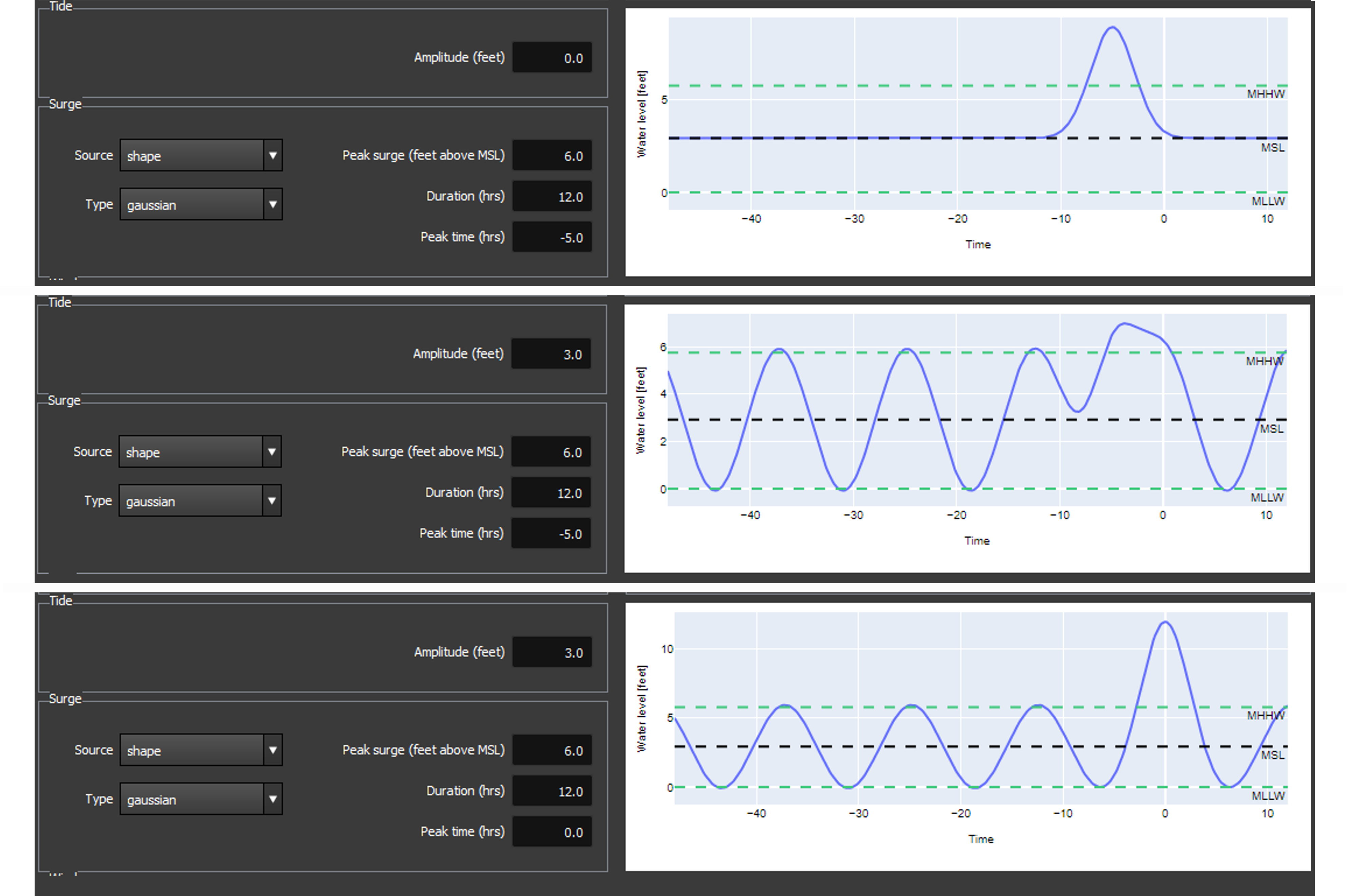
There are several datums shown in the water level plot: mean lower low water (MLLW), mean sea level (MSL), and mean higher high water (MHHW). The zero point, which is set to mean lower low water (MLLW) in Figure 3, is configurable and chosen at system set-up to be most intuitive for the intended users of the system.
Rainfall
For a synthetic event, can choose none (this is the default option), a constant intensity that will be applied over the entire duration of the event, or a shape, which is a rainfall timeseries based on standard curves.
Rainfall curves
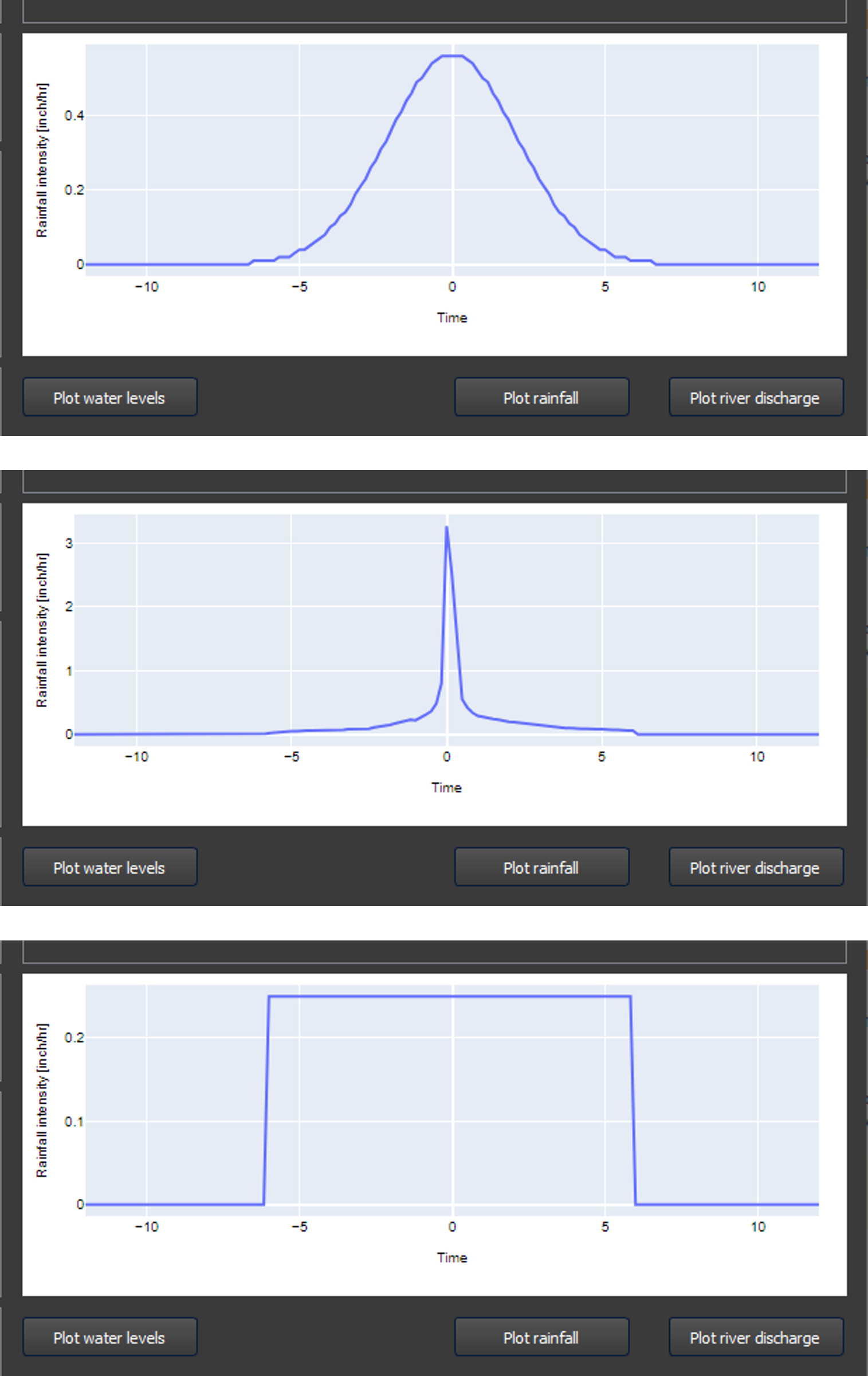
There are three rainfall curves that a user can select to specify the rainfall timeseries:
Gaussian - this is a Gaussian curve where the user specifies the cumulative rainfall, the duration of the rainfall, and the peak time of the rainfall relative to T=0.
Block - this is a rectangular shaped curve, which represents constant rainfall intensity over a specified duration. The user specifies the cumulative rainfall and the start and stop time of the rainfall in hours relative to T=0.
SCS - These curves are often used in practice in the US, and were developed by the Soil Conservation Service (SCS), now known as the National Resources Conservation Service. There are three SCS rainfall curves for different parts of the US. The curve that a user can select in the event teplate window will already be configured for the site location (part of system set-up). The user specifies the cumulative rainfall, the duration of the rainfall, and the start time in hours (relative to T=0).
Wind
For a synthetic event, the user can only enter either none (default), or a constant wind speed. When entering a constant wind speed, the user is asked to enter both the wind speed and wind direction. The direction should be entered in nautical degrees. This represents the direction where the wind is coming from. A direction of 0 degrees means wind is blowing from the North, 90 degrees means wind is blowing from the East.
River discharge
The river discharge represents the discharge in a river at the model boundary. If there are multiple rivers at the model boundary, the user will be able to select each river to specify the discharge. The user has two options for specifying the river discharge: a constant discharge or a shape, which is a synthetic timeseries.
Constant - A constant discharge is the default option. An average discharge value is filled in, which is specified in a FloodAdapt configuration folder at system setup. The user can change the value of the constant discharge.
Shape - The shape option uses a Gaussian curve. The user must specify the base discharge (this can be left at the default value, which is the average discharge), a peak discharge, a duration, and a peak time. The duration refers to the duration that the river discharge is above its base value.